Model 2019 Base-Year Updates

The following parameters and inputs were updated to bring the WF TDM base year from 2015 to 2019.

Parameters

Income

Median income parameters for the model were updated using 2019 5-year ACS data and kept in 2019 dollars to reflect 2019 base year. Median income parameters in version 8 were estimated from 2015 ACS data and deflated to 2010 dollars. The regional median income was calculated for each county and for each model space and used to update the following income-related parameters in 0_GeneralParameters.block.

Table 1: Regional Median Income

Parameter	v9 Value	v8 Value
Reg_Median_Inc	$74,946	$58,793

Table 2: Income Break Points for Airport Exogenous Trip Table Generation

Parameter	v9 Value	v8 Value	Notes
Income_Lo	$45,000	$35,000	breakpoint between Inc1 & Inc2
Income_Md	$75,000	$70,000	breakpoint between Inc2 & Inc3
Income_Hi	$125,000	$100,000	breakpoint between Inc3 & Inc4

The TAZ-level median income was also updated within the socioeconomic input files.

The household disaggregation income lookup curves and seed table were re-estimated based on the 2019 ACS data. The income lookup curves were estimated using data for all of Utah then calibrated specifically for the Wasatch Front model. Figure 1 shows a comparison of the version 9 and version 8 income lookup curves for the Wasatch Front.

The version 9 calibrated curves show a slight shift in the proportion of households toward the highest income groups from the middle two income groups relative to version 8. The lowest income group was very similar between versions 8 and 9. As the model currently groups the top three income groups into the “high income” category, the impact to the model is minimal.

Figure 1: Comparison of Wasatch Front Income Lookup Curves

Value of Time

Value of time parameters were updated using 2019 5-year ACS data. The value of time calculation in version 9 used the same assumptions as version 8 (i.e. 39% of median income for work trips, 30% of median income for personal trips, etc.). The value of time parameters in version 9 are in 2019 dollars. Version 8 parameters were calibrated to 2015 ACS data and deflated to 2010 dollars. Values of time are in cents/minute.

Table 3: Value of Time Rates

v9 Parameter	v9 Value	v8 Parameter	v8 Value	Notes
VOT_Auto_Wrk	22	VOT_Auto_Wrk	18	work trips (HBW)
VOT_Auto_Per	17	VOT_Auto_Per	14	non-work trips
VOT_Auto_Ext	20	VOT_Auto_Ext	16	external
VOT_LT	37	VOT_LT	30	light truck
VOT_MD	50	VOT_MD	40	medium truck
VOT_HV	63	VOT_HV	50	heavy truck
VOT_Toll	63	VOT_Toll	50	all vehicles on tollway
VOT_HOT_DA	63	VOT_HOT_DA	50	drive alone on HOT

To better understand the relative change in the value of time parameters, the parameters were normalized by the work-trip parameter and the percent difference in the ratios was compared. The percent differences show that the relative change between the variables in versions 8 and version 9 is very similar, indicating there isn’t a strong behavioral change due to the update of this parameter.

Table 4: Relative Value of Time Ratios

Category	v9 Value Relative to Work Trips	v8 Value Relative to Work Trips	% Difference
work trips	1	1	0.0%
non-work trips	0.77	0.78	-0.6%
external	0.91	0.89	2.3%
light truck	1.68	1.67	0.9%
medium truck	2.27	2.22	2.3%
heavy truck	2.86	2.78	3.1%

Auto Operating Costs

Auto operating costs were updated to reflect 2019 fuel cost, average fuel economy, and cost of vehicle maintenance and are in 2019 dollars. Version 8 parameters were calibrated to 2015 data and deflated to 2010 dollars. Costs are in cents/mile.

Table 5: Auto Operating Cost Parameters

Parameter	v9 Value	v8 Value	Notes
AOC_Auto	21.7	18.3	auto
AOC_LT	27.3	24.6	light truck
AOC_MD	55.5	47.8	medium truck
AOC_HV	74.3	63.7	heavy truck

The auto operating cost parameters in versions 8 and 9 were normalized by the auto-cost parameter. The percent differences between the version 8 and 9 ratios indicate that the relative cost to operate trucks compared to autos is slightly less in version 9 than in version 8.

Table 6: Relative Auto Operating Cost Ratios

Category	v9 Value	v8 Value	% Difference
auto	1	1	0.0%
light truck	1.26	1.34	-6.4%
medium truck	2.56	2.61	-2.1%
heavy truck	3.42	3.48	-1.6%

The relationship (ratio) between the auto operating costs and the value of time affects the distance term in the best-path functions in the distribution and assignment models. The higher the ratio, the more influence the distance term will exhibit on path choice and the more the model will be sensitive to shortest path vs. shortest time. A comparison of the ratios suggests that, while the overall pattern looks similar, distance will have slightly less influence on path choice for person trips in version 9 than in version 8, meaning person trips will be slightly more sensitive to congestion (i.e. travel time). This slight difference, however, should not be large enough to fundamentally change the behavior in the model. There is a more significant difference in the ratio for truck trips suggesting that truck trips (in particular light trucks) will be a little more sensitive to the influence of congestion in version 9 than in version 8.

Table 7: Auto Operating Cost / Value of Time Ratios

Category	v9 Value	v8 Value	% Difference
work trips	0.986	1.017	-3.0%
non-work trips	1.276	1.307	-2.3%
external	1.085	1.144	-5.1%
light truck	0.738	0.82	-10.0%
medium truck	1.11	1.195	-7.1%
heavy truck	1.179	1.274	-7.4%

Managed Lane Costs

Peak and off-peak toll cost parameters for tollways (FT=40) were updated to 48 cents/mile. This equates to approximately $5.00 for work trips (using an average work trip distances of 10.25) and $3.00 for non-work trips (using an average distance of 6.5 miles).

Peak toll cost parameters for HOT lanes (FT=38) and reliability lanes were updated to 34 cents/mile. This equates to approximately $3.50 for work trips and $2.20 for non-work trips (using the same average distances for work and non-work trips). Off-peak toll cost parameters were set as half the peak cost.

Version 9 tolls are in 2019 dollars. Toll costs for version 8 are in 2010 dollars.

Table 8: Managed Lane Cost Rates

Parameter	v9 Value	v8 Value	Notes
Cost_Toll_Pk	48	24	Tollways (FT 40) cost - Peak
Cost_Toll_Ok	48	24	Tollways (FT 40) cost - Off-peak
Cost_HOT_Pk	34	10	HOT (FT 38) cost - Peak
Cost_HOT_Ok	17	5	HOT (FT 38) cost - Off-peak
Cost_REL_Pk	34	10	Reliability lane cost - Peak
Cost_REL_Ok	17	5	Reliability lane cost - Off-peak

Relative to HOT toll costs, tollway costs are approximately 40% lower in version 9 than version 8, suggesting tollways would have less sensitivity to cost in version 9 than version 8. However, there are no tollways planned in the 2023 RTP.

Parking Costs

The permanent and temporary cost fields, PRKCSTPERM and PRKCSTTEMP located in the 1_Inputs\1_TAZ\TAZ.shp shapefile, were updated to reflect current conditions. Costs for parking in the downtown areas of Salt Lake City, Ogden, and Provo and around the universities were based on 2022 parking rates obtained from the city of Salt Lake City, web searches, and field visits.

The temporary parking cost for the Salt Lake City International Airport was set to $1.25 based on a weighted average of short-term premium and economy rates. This represents a $0.25 (25%) increase from version 8. Permanent parking costs were kept at $0 as workers at the airport do not pay for parking.

The Lagoon temporary parking cost was set to $6 based on the 2022 advertised parking rate of $18 per day by an assumed average occupancy of 3 people per vehicle. This represents a $1 (20%) increase from version 8. Permanent parking costs were kept at $0 as workers at Lagoon do not pay for parking.

Version 9 parking costs are in 2019 dollars, whereas version 8 parking costs are in 2010 dollars.

Transit Fares

Version 9 transit fares in the PT_Parameter\GENERAL_Fare.FAR file in the scenario line folder were updated to reflect the 2019 full advertised fares. This represented a two-fold change to the transit fares parameter. Previous models have fares coded as “average discounted fares” which included discounts for monthly passes, education passes, fare-pay, senior discounts, employer paid passes, and other discounts. In order to make updating transit fares in the model easier and more intuitive, the input fares were kept as full advertised fares and the calculation from advertised to discounted fares is now processed in the model stream.

Version 9 uses the same average discount assumptions as version 8. The transit fare discount was calculated in previous models to be 46% off the advertised fare yielding a discounted fare rate of 54% and the following parameter was added to the 0_GeneralParameters.block:

• FARE_DISCOUNT = 0.54

Bus Speed Ratios

An effort was made to refresh the bus speed factors in version 9. General transit feed specification (GTFS) data for 2019 was used to re-evaluate the version 8 bus speed ratio classifications and to estimate new bus speed ratios. The number of bus speed ratios were expanded from 6 in version 8 to 50 in version 9. The new ratios include more area type classifications as well as a classification for peak and off-peak. The bus speed ratios for versions 8 and 9 can be seen in Figure 2.

Bus speed ratio parameters were removed from the 0_GeneralParameters.block file in version 9 and are now read in via an input file (1_Inputs\0_GlobalData\4_ModeChoice\bus_speed_ratios.csv). A source spreadsheet (_source - bus_speed_ratios.xlsx) is also included in the input folder. Modifications to the transit skim script were made to incorporate the new bus speeds input file.

Bus Speed Ratios Plot

Code

faDataBusSpeeds     = FileAttachment("data\\bus_speed_ratios_long.csv").csv({ typed: true });
faFunctionalClasses = FileAttachment("data\\functionalclass.csv"      ).csv({ typed: true });
faTimePeriods       = FileAttachment("data\\timeperiod.csv"           ).csv({ typed: true });
faAreaTypes         = FileAttachment("data\\areatype.csv"             ).csv({ typed: true });

viewof facetSelect  = Inputs.select(new Map([['Time Period', 'TimePeriodName'], ['Area Type', 'AreaTypeName'], ['Functional Class', 'FunctionalClassName']]), {value: 'TimePeriodName'     , label: "Columns:"});
viewof domainSelect = Inputs.select(new Map([['Time Period', 'TimePeriodName'], ['Area Type', 'AreaTypeName'], ['Functional Class', 'FunctionalClassName']]), {value: 'AreaTypeName'       , label: "X-Axis:"});
viewof strokeSelect = Inputs.select(new Map([['Time Period', 'TimePeriodName'], ['Area Type', 'AreaTypeName'], ['Functional Class', 'FunctionalClassName']]), {value: 'FunctionalClassName', label: "Series:"});

// FILTER DATA
//viewof functionalclasses_checked = Inputs.checkbox(faFunctionalClasses.map(function(d) {return d.FunctionalClassName}),
//                                                   {value: faFunctionalClasses.map(function(d) {return d.FunctionalClassName}),
//                                                    label: "Function Class"});
//viewof timeperiods_checked       = Inputs.checkbox(faTimePeriods      .map(function(d) {return d.TimePeriodName     }),
//                                                   {value: faTimePeriods      .map(function(d) {return d.TimePeriodName     }),
//                                                    label: "Time Period"   });
//filteredBusData = faDataBusSpeeds.filter(function(busspeed) {
//  return functionalclasses_checked.includes(busspeed.FunctionalClassName) &&
//         timeperiods_checked      .includes(busspeed.TimePeriodName     )// &&
//         //areatypes        .includes(busspeed.AreaTypeName  );
//});

domainFromSelect = {
  switch(domainSelect) {
    case 'TimePeriodName'     : return faTimePeriods      .map(function(d) {return d.TimePeriodName     }); break;
    case 'AreaTypeName'       : return faAreaTypes        .map(function(d) {return d.AreaTypeName       }); break;
    case 'FunctionalClassName': return faFunctionalClasses.map(function(d) {return d.FunctionalClassName}); break;
    default: return;
  }
}

//xPlotDomainSelect = {
//  switch(domainSelect) {
//    case 'TimePeriodName'     : return "TimePeriod"     ; break;
//    case 'AreaTypeName'       : return "AreaType"       ; break;
//    case 'FunctionalClassName': return "FunctionalClass"; break;
//    default: return;
//  }
//}

fLabel = {
  switch(facetSelect) {
    case 'TimePeriodName'     : return "Time Period"     ; break;
    case 'AreaTypeName'       : return "Area Type"       ; break;
    case 'FunctionalClassName': return "Functional Class"; break;
    default: return;
  }
}

xLabel = {
  switch(domainSelect) {
    case 'TimePeriodName'     : return "Time Period"     ; break;
    case 'AreaTypeName'       : return "Area Type"       ; break;
    case 'FunctionalClassName': return "Functional Class"; break;
    default: return;
  }
}

domainFacetSelect = {
  switch(facetSelect) {
    case 'TimePeriodName':
      return faTimePeriods.map(function(d) {
          return d.TimePeriodName
        });
      break;
    case 'AreaTypeName':
      return faAreaTypes.map(function(d) {
          return d.AreaTypeName
        });
      break;
    case 'FunctionalClassName':
      return faFunctionalClasses.map(function(d) {
          return d.FunctionalClassName
        });
      break;
    default:
      return; 
  }
}

Code

Plot.plot({
  grid: true,
  aspectRatio: 0.25,
  facet: { data: faDataBusSpeeds, x: facetSelect, label: fLabel, marginTop: 40},
  x: {
    label: xLabel,
    domain: domainFromSelect,
    tickSize: 4,
    tickPadding: 2,
    marginTop: 40,
    tickRotate: 90,
  },
  y: {
    label: "Bus Speed Ratio",
    domain: [0, 1],
    fontSize: 8
  },
  color: { type: "categorical", legend: true, legendStyle: { fontSize: 16 } },
  style: {
    fontSize: 12
  },
  marginTop: 60,
  marginBottom: 120,
  marks: [
    Plot.frame(),
    Plot.line(faDataBusSpeeds, { x: domainSelect, y: "BusSpeedRatio", stroke: strokeSelect, strokeWidth: 2 }),
    Plot.dot(faDataBusSpeeds, { x: domainSelect, y: "BusSpeedRatio", stroke: strokeSelect, r: 4, fill: strokeSelect })
  ]
})

Figure 2: Bus Speed Ratios

Bus Speed Ratios Data

Code

Inputs.table(faDataBusSpeeds, {
  style: {
    fontSize: 12,
  },
  columns: [
    "FunctionalClassName",
    "TimePeriodName",
    "AreaTypeName",
    "BusSpeedRatio"
  ],
  header: {
    FunctionalClassName: "Functional Class",
    TimePeriodName: "Time Period",
    AreaTypeName: "Area Type",
    BusSpeedRatio: "Bus Speed Ratio"
  }
})

Previous Bus Speed Ratios

Code

// read in CSVs
faDataBusSpeeds_previous = FileAttachment("data\\bus_speed_ratios_previous.csv").csv({ typed: true });

Code

Plot.plot({
  grid: true,
  aspectRatio: 0.5,
  style: {
    fontSize: 12,
  },
  margin: 40,
  marginBottom: 150,
  x: {
    label: "",
    //tickFormat: () => "",
    tickRotate: 90,
    domain: faDataBusSpeeds_previous.map(function(d) {return d.FunctionalClass}),
    tickSize: 0
  },
  y: {label: "Bus Speed Ratio" , domain: [0, 1]},
  color: { type: "categorical", legend: false },
  marks: [
    Plot.frame(),
    Plot.barY(faDataBusSpeeds_previous, {x: "FunctionalClass", y: "BusSpeedRatio", stroke: "FunctionalClass", fill: "FunctionalClass"})
  ]  
})

Figure 3: Previous Bus Speed Ratios

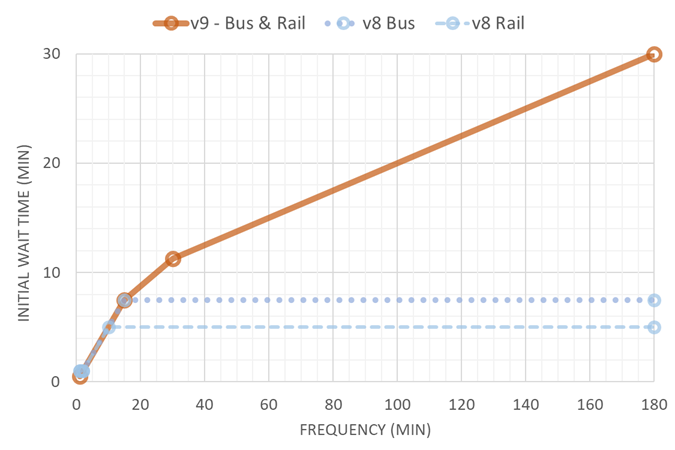
Initial Wait Time

The initial wait time curves found in 1_Inputs\4_Transit\Lin_2019\PT_Parameter\GENERAL_System.PTS were updated in version 9 to make the mode choice model more sensitive to frequency changes. Version 8 initial wait time curves were based on the premise that transit patrons are familiar with the transit schedule and plan their trip to initially board with the minimum amount of delay. To reflect this behavior, a 7.5-minute cap for bus and a 5-minute cap for rail was set on the initial wait time parameter. This cap, however, caused the model to not see much of the benefit/disbenefit a transit user would experience when headways are changed, in particular for longer when moving away/to longer headways.

The version 9 initial wait time parameter was set based on research given to UTA of industry standard-practice initial wait time curves. A range of initial wait time curve values were presented in the research. Version 9 was calibrated to a more conservative curve in that range. The version 9 initial wait time curve can be seen in Figure 4.

The new initial wait time curve in version 9 had the effect of increasing transit ridership relative to version 8 in scenarios where an investment in more frequent transit was projected. Early testing showed this increase to be on the order of magnitude of 8-12% based on a comparison of 2019 RTP and draft 2023 RTP transportation investments. However, the actual change in ridership would vary depending on the initial starting point and the magnitude of change in transit frequency.

Figure 4: Initial Wait Time Curve

Auto Occupancy

Auto occupancy variables were expanded to include additional trips purposes. New auto occupancy rates were calculated based on 2012 Household Travel Survey records for just the Wasatch Front model space. Auto-occupancy rates for external trips are the average of internal-external and external-internal trips. The new version 9 auto occupancy rates can be found in Table 9 and Table 9.

Table 9: Vehicle Occupancy Rates

v9 Parameter	v9 Value	v8 Parameter	v8 Value	Notes
VehOcc_HBW	1.1	VEH_OCCUPANCY_HBW	1.1	Home-Based Work
VehOcc_HBShp	1.63	VEH_OCCUPANCY_HBSHP	1.58	Home-Based Shopping
VehOcc_HBOth	1.68	VEH_OCCUPANCY_HBOTH	1.66	Home-Based Other
VehOcc_HBSch	1.76	VEH_OCCUPANCY_HBSCH	2.14	Home-Based School
VehOcc_HBC	1.12	VEH_OCCUPANCY_HBC	1.26	Home-Based College
VehOcc_NHBW	1.21	VEH_OCCUPANCY_NHBW	1.2	Non-Home-Based Work
VehOcc_NHBNW	1.76	VEH_OCCUPANCY_NHBNW	1.7	Non-Home-Based Non-Work
VehOcc_Rec	1.68	(Uses HBO)	1.64	Recreation
VehOcc_HBO	1.67	VEH_OCCUPANCY_HBO	1.64	Home-Based Other (HBShp+HBOth)
VehOcc_NHB	1.54	VEH_OCCUPANCY_NHB	1.48	Non-Home-Based (NHBW+NHBNW)
VehOcc_ExtWrk	1.16	(Uses HBW)	1.1	External Work
VehOcc_ExtHBO	1.82	(Uses HBO)	1.64	External Home-Based Other
VehOcc_ExtNHB	1.73	(Uses NHB)	1.48	Non-Home-Based
VehOcc_ExtRec	1.73	(Uses HBO)	1.64	External Recreation

Table 10: Vehicle Occupancy 3+ Rates

v9 Parameter	v9 Value	v8 Parameter	v8 Value	Notes
VehOcc_3p_HBW	3.53	VEH_OCC_3P_HBW	3.4	3+ Person Home-Based Work
VehOcc_3p_HBShp	3.49	(Uses HBO)	3.55	3+ Person Home-Based Shopping
VehOcc_3p_HBOth	3.73	(Uses HBO)	3.55	3+ Person Home-Based Other
VehOcc_3p_HBSch	3.88	(Uses HBO)	3.55	3+ Person Home-Based School
VehOcc_3p_HBC	3.24	VEH_OCC_3P_HBC	3.53	3+ Person Home-Based College
VehOcc_3p_NHBW	3.71	(Uses NHB)	3.51	3+ Person Non-Home-Based Work
VehOcc_3p_NHBNW	3.71	(Uses NHB)	3.51	3+ Person Non-Home-Based Non-Work
VehOcc_3p_Rec	3.73	(Uses HBO)	3.55	3+ Person Recreation
VehOcc_3p_HBO	3.68	VEH_OCC_3P_HBO	3.55	3+ Person Home-Based Other (HBShp+HBOth)
VehOcc_3p_NHB	3.71	VEH_OCC_3P_NHB	3.51	3+ Person Non-Home-Based (NHBW+NHBNW)

Other Input Files

K-12 School Enrollment

The kindergarten through 12th grade (K-12) school enrollment fields, Enrol_Elem, Enrol_Midl, and Enrol_High located in the socioeconomic input files, were updated using the 2019 statewide school enrollment database. This was done at the state-wide level and then applied to the Wasatch Front region. Additionally, a point shapefile of the state-wide dataset is included with the TDM, as shown in Figure 5.

Code

L = require('leaflet@1.2.0')
html`<link href='${resolve('leaflet@1.2.0/dist/leaflet.css')}' rel='stylesheet' />`

Code

geojsonK12Enroll = FileAttachment("data/k12enroll.geojson").json()

Code

mapK12Enroll = {

  let container = DOM.element('div', { style: `width:${width}px;height:${width/1.6}px` });
  yield container;
  
  let map = L.map(container).setView([40.7608, -111.8910], 8.25);

  let greyLayer = L.tileLayer('https://{s}.basemaps.cartocdn.com/light_all/{z}/{x}/{y}{r}.png', {
    attribution: '&copy; <a href="https://www.openstreetmap.org/copyright">OpenStreetMap</a> contributors'
  }).addTo(map);

  var cHigh = "#FF0000"
  var cMidl = "#00FF00"
  var cElem = "#0000FF"

  var geojsonMarkerOptions_High = {
      radius: 4,
      fillColor: cHigh,
      color: cHigh,
      weight: 2,
      opacity: 1,
      fillOpacity: 1.0,
  };

  var geojsonMarkerOptions_Midl = {
      radius: 4,
      fillColor: cMidl,
      color: cMidl,
      weight: 2,
      opacity: 1,
      fillOpacity: 1.0,
  };
  var geojsonMarkerOptions_Elem = {
      radius: 4,
      fillColor: cElem,
      color: cElem,
      weight: 2,
      opacity: 1,
      fillOpacity: 1.0,
  };
            
  // function to use different icons based on number of stations
  function markerByEnrollment(feature) {
    if (feature.properties.Enrol_High >= 100) {
      return geojsonMarkerOptions_High
    } else if (feature.properties.Enrol_Midl >= 100){
      return geojsonMarkerOptions_Midl;
    } else{
      return geojsonMarkerOptions_Elem;
    }
  };

  function getColor(c) {
    if (c=='High School') {
      return cHigh;
    } else if (c=='Middle School') {
      return cMidl;
    } else if (c=='Elementary School') {
      return cElem;
    }
  };
          
  // create the GeoJSON layer and call the styling function with each marker
  var layerSchools = L.geoJSON(geojsonK12Enroll,  {
    pointToLayer: function (feature, latlng) {
      var mypopup = L.popup().setContent("<b>" + feature.properties.SchoolName + " Enrollment</b>" +
                    "<br><b>High School: </b>" + feature.properties.Enrol_High +
                    "<br><b>Middle School: </b>" + feature.properties.Enrol_Midl +
                    "<br><b>Elementary School: </b>" + feature.properties.Enrol_Elem);
      var mymarker = L.circleMarker(latlng, markerByEnrollment(feature));
      mymarker.bindPopup(mypopup);
      return mymarker;
    }
  }).addTo(map);

  var legend = L.control({position: 'bottomleft'});
    legend.onAdd = function (map) {
      var div = L.DomUtil.create('div', 'info legend');
      var labelsBill = []; // legend title
      var lcategories = ['High School','Middle School','Elementary School'];

      for (var i = 0; i < lcategories.length; i++) {
        div.innerHTML += 
          labelsBill.push(
            '<i class="bi bi-circle-fill" style="color:' + getColor(lcategories[i]) + '"></i> ' +
          (lcategories[i] ? lcategories[i] : '+'));
      }
      div.innerHTML = labelsBill.join('<br>');

      // Add CSS style for the background color
      div.style.backgroundColor = 'lightgray';
      div.style.padding = '10px';
      
      return div;
    };
    legend.addTo(map);

  //let lyrK12Enroll = L.geoJson(geojsonK12Enroll, { size: 5, color: '#FFFFFF'}).addTo(map);
  
}

Figure 5: K-12 School Locations

College Enrollment

Base Distribution

The college student base-year distribution located in 1_Inputs\0_GlobalData\0_TripTables\BaseDistribution.csv was updated to reflect current conditions. Dormitory populations were assigned to TAZs based on group quarter data from the Census. The remaining enrollment was distributed using StreetLight origin-destination and USHE enrollment data.

Enrollment Forecast

The future-year college enrollment control totals located in 1_Inputs\0_GlobalData\0_TripTables\TripTableControlTotal.csv were updated to reflect current USHE and other college enrollment data. Colleges that were “removed” in version 9 had the college enrollment control total set to zero. A comparison of the version 9 and version 8 (specifically, version 8.3.2) college enrollment control totals can be seen in Figure 6.

Code

collegeT = transpose(dfcollege)

optionsColleges = 
[
  ['LDS Business College', 'LDSBC'],
  ['Westminster', 'Westmin'],
  ['UofU Main Campus', 'UofU_Main'],
  ['UofU Medical', 'UofU_Med'],
  ['WSU Main Campus', 'WSU_Ogden'],
  ['WSU Davis', 'WSU_Davis'],
  ['WSU West Campus', 'WSU_West'],
  ['SLCC Main Campus', 'SLCC_TL'],
  ['SLCC South City', 'SLCC_SC'],
  ['SLCC Jordan', 'SLCC_JD'],
  ['SLCC Meadowbrook', 'SLCC_Mead'],
  ['SLCC Miller', 'SLCC_ML'],
  ['SLCC Library', 'SLCC_LB'],
  ['SLCC Hiland', 'SLCC_HL'],
  ['SLCC Airport', 'SLCC_Airp'],
  ['SLCC Westpoint', 'SLCC_West'],
  ['SLCC Herriman', 'SLCC_HM'],
  ['BYU', 'BYU'],
  ['UVU Main Campus', 'UVU_main'],
  ['UVU Geneva', 'UVU_Geneva'],
  ['UVU Lehi', 'UVU_ThankP'],
  ['UVU Vineyard', 'UVU_VINE'],
  ['UVU Payson', 'UVU_PAYSON']]

viewof selectCollege = Inputs.select(new Map(optionsColleges), {value: 'LDSBC', label: 'College: '});

// FILTER DATA
college_v98= collegeT.filter(function(collegeData) {
  return selectCollege   == collegeData.College
});

college_v9= collegeT.filter(function(collegeData) {
  return selectCollege   == collegeData.College &&
  'v9' == collegeData.Version; 
});

college_v8= collegeT.filter(function(collegeData) {
  return selectCollege   == collegeData.College &&
  'v832' == collegeData.Version; 
});

maxY1 = Math.max(...college_v98.map(item => item.Enrollment));

Code

html`<html lang="en">
<head>
    <meta charset="UTF-8">
    <meta name="viewport" content="width=device-width, initial-scale=1.0">
    <title>Version Display</title>
    <style>
        .green-text {
            color: green;
            font-size: 12px;
            font-weight: bold;
            padding-left: 60px;
        }

        .blue-text {
            color: #376092;
            font-size: 12px;
            font-weight: bold;
            padding-left: 20px;
        }
    </style>
</head>
<body>
    <span class="green-text"> —— Version 8</span>
    <span class="blue-text"> —— Version 9</span>
</body>
</html>`

Code

Plot.plot({
  grid: true,
  aspectRatio: 0.5,
  x: { label: 'Year', tickFormat: d => d },
  y: { label: 'Enrollment', tickFormat: f => f, domain: [0, maxY1] },
  marginRight: 60,
  marginLeft: 60,
  style: {
    fontSize: 15
  },
  marginTop: 10,
  marginBottom: 60,
  marks: [
    Plot.line(
      college_v9, { x: 'Year', y: 'Enrollment', stroke: "#376092", strokeWidth: 4, color: { legend: 'Version' } }),
    Plot.line(
      college_v8, { x: 'Year', y: 'Enrollment', stroke: "#77933c", strokeWidth: 4, color: { legend: 'Version' } }),
    Plot.frame({ strokeOpacity: 0.2 }),
  ]
});

Figure 6: College Enrollment Forecasts

College Enrollment Factors

The college enrollment factors located in 1_Inputs\0_GlobalData\0_TripTables\College_Factors.csv were updated in association with the college enrollment control totals.

• % Removed – For colleges that were removed, the factor was reset to zero.
• Full-Time Equivalent (FTE) – the FTE rate was reduced for all colleges. This will have the effect of increasing the number of college students in the HBC college trip table. For colleges that were removed, the factor was reset to one.
• Home-Based-College (HBC) Trip Rate – For colleges that were removed, the factor was reset to zero.

A comparison of the version 9 and version 8 (specifically, version 8.3.2) college enrollment control totals can be seen in Table 11.

Table 11: College Enrollment Factors

Areas	Campus	% Removed v9 Value	% Removed v8 Value	FTE Rate v9 Value	FTE Rate v8 Value	HBC Trip Rate v9 Value	HBC Trip Rate v8 Value	Notes
WFRC Colleges	Ensign	0.101	0.101	1.179	1.179	0.93	0.93
	Westminster	0.012	0.012	1.098	1.098	0.93	0.93
	UofU Main	0.026	0.026	1.025	1.21	0.93	0.93
	UofU Med	0	0.026	1	1.21	0	0.93	(removed)
	WSU Main	0.215	0.215	1.038	1.588	0.83	0.83
	WSU Davis	0.309	0.309	1.038	1.588	0.677	0.677
	WSU West	0	0.309	1	1.588	0	0.677	(removed)
	SLCC Main	0.341	0.341	1.208	2.005	0.622	0.622
	SLCC South City	0.341	0.341	1.208	2.005	0.642	0.642
	SLCC Jordan	0.341	0.341	1.208	2.005	0.569	0.569
	SLCC Meadowbrook	0	0.341	1	2.005	0	0.569	(removed)
	SLCC Miller	0.341	0.341	1.208	2.005	0.616	0.616
	SLCC Library	0	0.341	1	2.005	0	0.616	(removed)
	SLCC Highland	0	0.341	1	2.005	0	0.616	(removed)
	SLCC Airport	0	0.341	1	2.005	0	0.616	(removed)
	SLCC Westpointe	0	0.341	1	2.005	0	0.616	(removed)
	SLCC Herriman	0	0.341	1	2.005	0	0.616	(removed)
MAG Colleges	BYU	0.026	0.026	1.025	1.21	0.93	0.93
	UVU Main	0.27	0.27	1.097	1.4	0.945	0.945
	UVU Geneva	0	0.27	1	1.4	0	0.945	(removed)
	UVU Lehi	0.27	0.27	1.097	1.4	0.945	0.945
	UVU Vineyard	0.27	0.27	1.097	1.4	0.945	0.945
	UVU Payson	0.27	0.27	1.097	1.4	0.945	0.945

Calibration

Trip Generation Rates

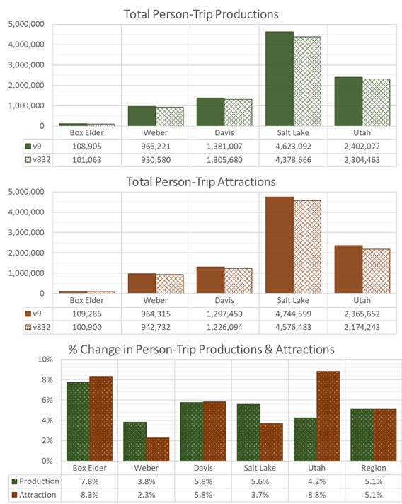
Trip generation rates were updated in version 9 as part of the model’s base year calibration. Person-trip production rates (e.g. HBW, HBShp, HBOth, etc.) were increased in the model script by approximately 5% over version 8 rates resulting in a regional increase of both productions and attractions of 5% (see Figure 7). County-level adjustments were left the same as the previous model. When combined with the changes in the 2019 socioeconomic data, the total person-trip productions and attractions in individual counites was slightly different with the most notable differences in Weber, Salt Lake, and Utah counties. The county production/attraction balance stayed fairly consistent.

Figure 7: Person-Trip Productions & Attractions by County

Short haul tuck calculations were revamped and simplified mirroring changes made to truck trip calculations in USTM. The moving people, goods, and services by light, medium, and heavy truck detailed calculations were collapsed to just light, medium, and heavy categories. (Note, the trip generation script still includes code for the more detailed calculations, however most of this code is not being used.) The new short haul truck trip variables and coefficients were combined based on the original code structure. The short haul truck trip rates were then adjusted by county. Significant changes were made to the county light, medium, and heavy truck adjustment factors resulting in a 34% increase in overall short haul truck productions and attractions. Light trucks accounted for the majority of this change with a regional increase of 50%. Medium trucks saw a regional increase of 29%. Heavy trucks decreased by 1%. In addition to the changes in regional truck trip ends and vehicle classification makeup, significant changes occurred in the county-level distribution of the trip ends with Salt Lake County truck trip ends held constant yielding more than twice the regional change in the other counties (see Figure 8).

Figure 8: Short Haul Truck Productions & Attractions by County

The changes to the short haul trip end calculations constitute a new behavioral model.

Distribution Friction Factors

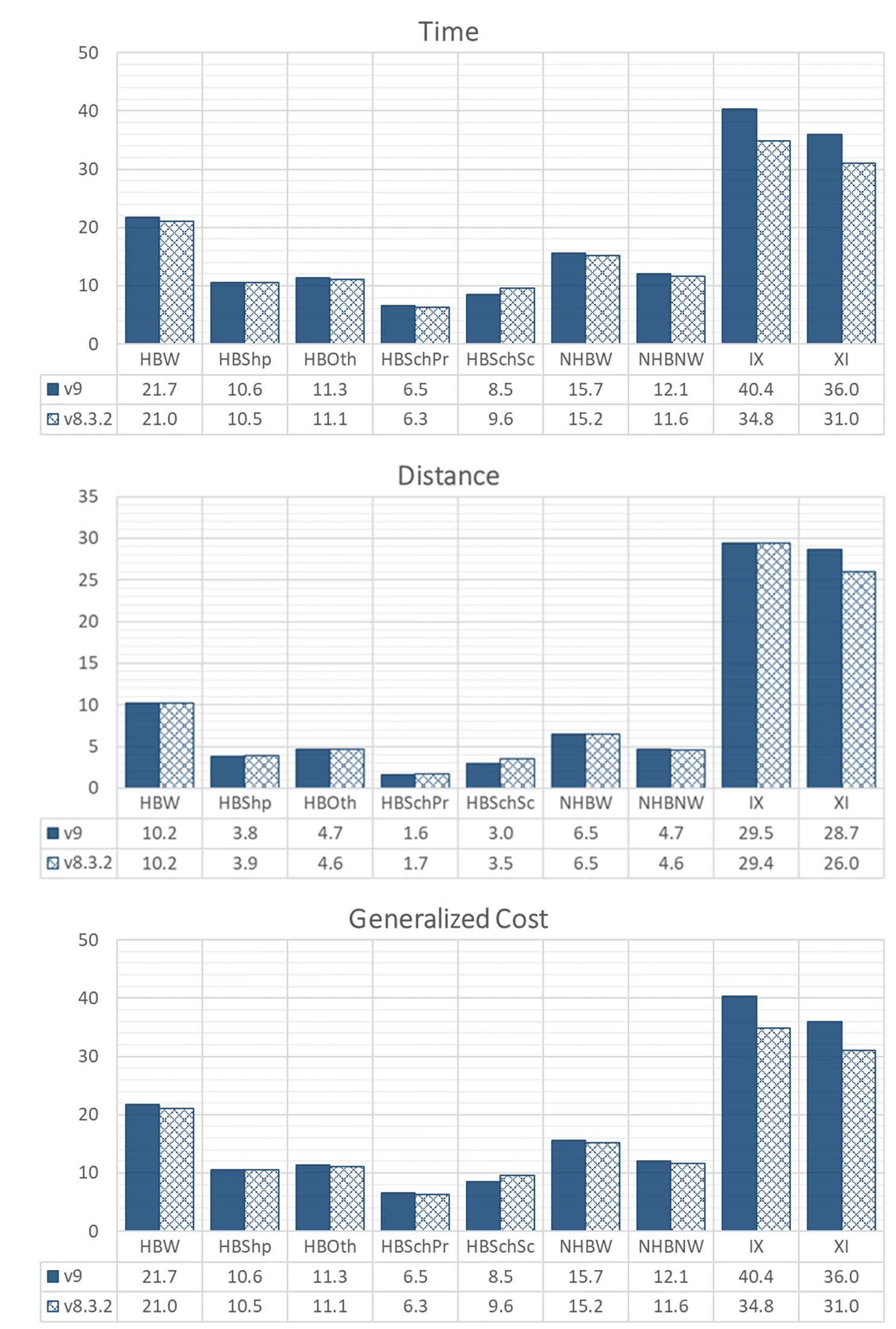
The observed time, distance, and generalized cost trip length frequencies and average trip lengths, which serve as the targets for friction factor calibration and validation, were updated in version 9 to reflect the 2019 base year network and refreshed data processing. The updated average trip length frequencies are found in Figure 9.

Figure 9: Observed Average Trip Length

Trip distribution friction factors were updated in version 9 as part of the model’s base year calibration. Six new external-truck friction factors were added: IX_LT, IX_MD, IX_HV, XI_LT, XI_MD, and XI_HV. Note however that IX_LT and XI_LT friction factors were set equal to IX and XI, respectively. StreetLight truck origin-destination data was used to help calibrate the internal truck and external friction factors. A comparison of the version 9 and version 8 friction factors is found in @figxx.

Code

ffT = transpose(dff)

optionsFF = 
[
  ['HBW', 'HBW'],   
  ['HBShp', 'HBShp'],
  ['HBOth', 'HBOth'],
  ['HBSch_Pr', 'HBSch_Pr'],
  ['HBSch_Sc', 'HBSch_Sc'],
  ['NHBW', 'NHBW'],
  ['NHBNW', 'NHBNW'],
  ['LT', 'LT'],
  ['MD', 'MD'],
  ['HV', 'HV'],
  ['IX', 'IX'],
  ['IX_LT', 'IX_LT'],
  ['IX_MD', 'IX_MD'],
  ['IX_HV', 'IX_HV'],
  ['XI',    'XI'],
  ['XI_LT', 'XI_LT'],
  ['XI_MD', 'XI_MD'],
  ['XI_HV', 'XI_HV']
]
 
viewof selectFF = Inputs.select(new Map(optionsFF), {value: 'HBW', label: 'Purpose: '});

// FILTER DATA
ff_v98= ffT.filter(function(ffData) {
  return selectFF == ffData.Purpose;
});

ff_v9= ffT.filter(function(ffData) {
  return selectFF == ffData.Purpose &&
  'v9' == ffData.Version; 
});

ff_v8= ffT.filter(function(ffData) {
  return selectFF   == ffData.Purpose &&
  'v832' == ffData.Version; 
});

Code

domainVals = [
    {Purpose: 'HBW',      X1MAX: 30, X2MIN: 20, X2MAX: 80 , X3MIN: 80 , X3MAX: 260, Y2MAX: .060, Y3MAX: .002  },
    {Purpose: 'HBShp',    X1MAX: 16, X2MIN: 15, X2MAX: 50 , X3MIN: 40 , X3MAX: 150, Y2MAX: .020, Y3MAX: .0003 },
    {Purpose: 'HBOth',    X1MAX: 16, X2MIN: 15, X2MAX: 50 , X3MIN: 40 , X3MAX: 150, Y2MAX: .020, Y3MAX: .0003 },
    {Purpose: 'HBSch_Pr', X1MAX: 10, X2MIN: 10, X2MAX: 40 , X3MIN: 40 , X3MAX: 100, Y2MAX: .003, Y3MAX: .00003},
    {Purpose: 'HBSch_Sc', X1MAX: 10, X2MIN: 10, X2MAX: 40 , X3MIN: 40 , X3MAX: 100, Y2MAX: .003, Y3MAX: .00003},
    {Purpose: 'NHBW',     X1MAX: 20, X2MIN: 20, X2MAX: 100, X3MIN: 100, X3MAX: 230, Y2MAX: .040, Y3MAX: .001  },
    {Purpose: 'NHBNW',    X1MAX: 20, X2MIN: 20, X2MAX: 100, X3MIN: 100, X3MAX: 230, Y2MAX: .040, Y3MAX: .001  },
    {Purpose: 'LT',       X1MAX: 10, X2MIN: 10, X2MAX: 60 , X3MIN: 60 , X3MAX: 120, Y2MAX: .040, Y3MAX: .001  },
    {Purpose: 'MD',       X1MAX: 10, X2MIN: 10, X2MAX: 60 , X3MIN: 60 , X3MAX: 120, Y2MAX: .040, Y3MAX: .001  },
    {Purpose: 'HV',       X1MAX: 10, X2MIN: 10, X2MAX: 60 , X3MIN: 60 , X3MAX: 120, Y2MAX: .040, Y3MAX: .001  },
    {Purpose: 'IX',       X1MAX: 80, X2MIN: 80, X2MAX: 200, X3MIN: 200, X3MAX: 300, Y2MAX: .060, Y3MAX: .03   },
    {Purpose: 'IX_LT',    X1MAX: 80, X2MIN: 80, X2MAX: 200, X3MIN: 200, X3MAX: 300, Y2MAX: .060, Y3MAX: .03   },
    {Purpose: 'IX_MD',    X1MAX: 80, X2MIN: 80, X2MAX: 200, X3MIN: 200, X3MAX: 300, Y2MAX: .060, Y3MAX: .03   },
    {Purpose: 'IX_HV',    X1MAX: 80, X2MIN: 80, X2MAX: 200, X3MIN: 200, X3MAX: 300, Y2MAX: .060, Y3MAX: .03   },
    {Purpose: 'XI',       X1MAX: 25, X2MIN: 20, X2MAX: 120, X3MIN: 80 , X3MAX: 280, Y2MAX: .080, Y3MAX: .008  },
    {Purpose: 'XI_LT',    X1MAX: 25, X2MIN: 20, X2MAX: 120, X3MIN: 80 , X3MAX: 280, Y2MAX: .080, Y3MAX: .008  },
    {Purpose: 'XI_MD',    X1MAX: 25, X2MIN: 20, X2MAX: 120, X3MIN: 80 , X3MAX: 280, Y2MAX: .080, Y3MAX: .008  },
    {Purpose: 'XI_HV',    X1MAX: 25, X2MIN: 20, X2MAX: 120, X3MIN: 80 , X3MAX: 280, Y2MAX: .080, Y3MAX: .008  }
]

domainFilter= domainVals.filter(function(data) {
  return selectFF == data.Purpose; 
});

x1max = domainFilter[0].X1MAX;
x2min = domainFilter[0].X2MIN;
x2max = domainFilter[0].X2MAX;
x3min = domainFilter[0].X3MIN;
x3max = domainFilter[0].X3MAX;
y2max = domainFilter[0].Y2MAX;
y3max = domainFilter[0].Y3MAX;

Code

html`<html lang="en">
<head>
    <meta charset="UTF-8">
    <meta name="viewport" content="width=device-width, initial-scale=1.0">
    <title>Version Display</title>
    <style>
        .green-text {
            color: green;
            font-size: 12px;
            font-weight: bold;
            padding-left: 60px;
        }

        .blue-text {
            color: #376092;
            font-size: 12px;
            font-weight: bold;
            padding-left: -20px;
        }
    </style>
</head>
<body>
    <span class="green-text"> —— Version 8</span>
    <span class="blue-text"> —— Version 9</span>
</body>
</html>`

Code

Plot.plot({
  grid: true,
  aspectRatio: 0.5,
  x: { label: 'Bin', tickFormat: d => d , domain:[0,x1max]},
  y: { label: 'Distribution', tickFormat: f => f, domain: [0, 1] },
  marginRight: 60,
  marginLeft: 60,
  color: { type: "categorical", legend: true, legendStyle: { fontSize: 23 } },
  style: {
    fontSize: 23
  },
  marginTop: 10,
  marginBottom: 60,
  height: 700,
  marks: [
    Plot.line(
      ff_v9, { x: 'Bin', y: 'Distribution', stroke: "#376092", strokeWidth: 4, color: { legend: 'Version' } }),
    Plot.line(
      ff_v8, { x: 'Bin', y: 'Distribution', stroke: "#77933c", strokeWidth: 4, color: { legend: 'Version' } }),
    Plot.frame({ strokeOpacity: 0.2 }),
      [
      Plot.text([`\n   ——   Current Projection \n\n   —  — Previous Projection`], {frameAnchor: "top-right", fontSize: 24})
  ]]
});
Plot.plot({
  grid: true,
  aspectRatio: 0.5,
  x: { label: 'Bin', tickFormat: d => d , domain:[x2min,x2max]},
  y: { label: 'Distribution', tickFormat: f => f, domain: [0, y2max] },
  marginRight: 60,
  marginLeft: 60,
  color: { type: "categorical", legend: true, legendStyle: { fontSize: 23 } },
  style: {
    fontSize: 23
  },
  marginTop: 10,
  marginBottom: 60,
  height: 700,
  marks: [
    Plot.line(
      ff_v9, { x: 'Bin', y: 'Distribution', stroke: "#376092", strokeWidth: 4, color: { legend: 'Version' } }),
    Plot.line(
      ff_v8, { x: 'Bin', y: 'Distribution', stroke: "#77933c", strokeWidth: 4, color: { legend: 'Version' } }),
    Plot.frame({ strokeOpacity: 0.2 }),
  ]
});
Plot.plot({
  grid: true,
  aspectRatio: 0.5,
  x: { label: 'Bin', tickFormat: d => d , domain:[x3min,x3max]},
  y: { label: 'Distribution', tickFormat: f => f, domain: [0, y3max] },
  marginRight: 60,
  marginLeft: 60,
  color: { type: "categorical", legend: true, legendStyle: { fontSize: 23 } },
  style: {
    fontSize: 23
  },
  marginTop: 10,
  marginBottom: 60,
  height: 700,
  marks: [
    Plot.line(
      ff_v9, { x: 'Bin', y: 'Distribution', stroke: "#376092", strokeWidth: 4, color: { legend: 'Version' } }),
    Plot.line(
      ff_v8, { x: 'Bin', y: 'Distribution', stroke: "#77933c", strokeWidth: 4, color: { legend: 'Version' } }),
    Plot.frame({ strokeOpacity: 0.2 }),
  ]
});

(a) Beginning of Curve

(b) Middle of Curve

(c) End of Curve

Figure 10: Friction Factors

K-Factors

K-factor variables were expanded by trip purpose to allow for more flexibility in calibrating the distribution model. However, no K-factors were needed for calibration. All K-factors were reset to 1.

Table 12: Reset K-Factors

Area	v9 Parameter	v9 Value	v8 Parameter	v8 Value
between Salt Lake and Utah counties	SL_UT_KFAC_Wrk	1	SL_UT_KFAC	0.85
	SL_UT_KFAC_Oth	1
	SL_UT_KFAC_Trk	1
	SL_UT_KFAC_Ext	1
between Salt Lake and Davis counties	SL_DA_KFAC_Wrk	1	SL_DA_KFAC	0.95
	SL_DA_KFAC_Oth	1
	SL_DA_KFAC_Trk	1
	SL_DA_KFAC_Ext	1
between Box Elder and Weber counties	WE_BE_KFAC_Wrk	1	WE_BE_KFAC	1.00
	WE_BE_KFAC_Oth	1
	WE_BE_KFAC_Trk	1
	WE_BE_KFAC_Ext	1

Mode Choice Constants

Mode choice constants were updated in version 9 as part of the model’s base year calibration.

In addition, the parameter used to set the Core Bus constant was renamed and lowered to 0.33. The effect of this change makes mode 5 in the model a little less attractive in version 9 than it was in version 8.

Table 13: Core Bus Constant Multiplier

v9 Parameter	v9 Value	v8 Parameter	v8 Value	Notes
RAIL2COR_MULTIPLIER	0.33	RAIL2BRT_MULTIPLIER	0.4	factor to set Core Route constant relative to LRT constant

Adjustment factors were added to the mode choice logit model to adjust CRT ridership in Davis and Utah counties. The parameters are applied in the utility calculation and represent a penalty/incentive in equivalent minutes.